How to Make a Position Table in Excel

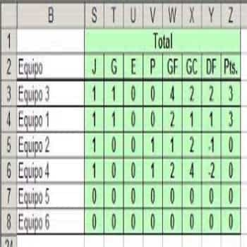
If you want to organize a large amount of information for later analysis, ranking, or study based on your results, you should create a leaderboard in Excel . With this tool, you could sort: sales figures per customer, student scores, tables with sports data, or record statistical information, among other options.

Steps to create a position table in Excel

Whether you want to study the results of sports competitions or determine who is the best salesperson in a company, there are many uses that you can give to this tool. This program offers you a simple and practical function exactly for this purpose. Here we show you in a simple way!

You might also be interested in: How to Create a Check Mark in Excel

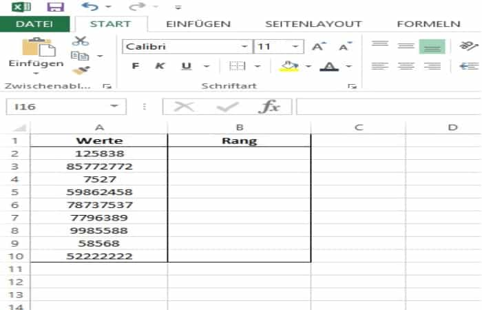
• Step 1: You type the values ​​into cells A2 through A10. The ranking list should appear in cells B2 through B10 (Note: The EQ RANK function which means "EQUAL CLASSIFICATION» is used to create the ranking list. In older versions of Excel, only «RANG» is now used.)

• Step 2: Click the mouse on the cell where the sort list starts. In this example B2.
• Step 3: Switch to the «Formulas» at the top and click the “Insert Function” button.
• Step 4: Choose "Global Data» as a category and «EQUAL CLASSIFICATION» as a function. If you confirm the process with «Accept» a new window will open.
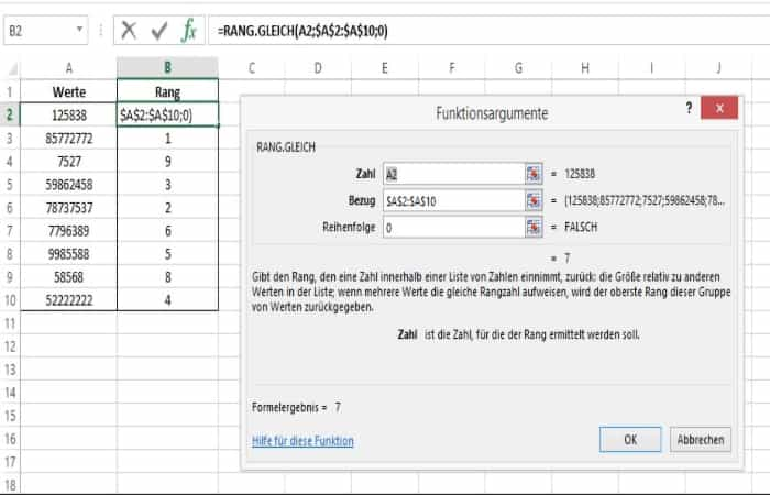
• Step 5: Click on the field «Number» and then select the top cell of the values. In this case A2.
• Step 6: Now mark the area between the first and last value in the field «Reference«. Here A2: A10.
• Step 7: If you press the key [F4], the reference is automatically converted to the appropriate format. A2:10 becomes the reference $A$2:$A$10.
• Step 8: If you enter 0 (zero) in the Order field, the highest value is ranked as 1. If you enter 1 instead of 0, the lowest value is ranked as 1.
• Step 9: If you close the window with the button «Accept", the first rank appears. If you simply drag the cell down, the entire ranking list will be created.

Sort items before making a leaderboard in Excel

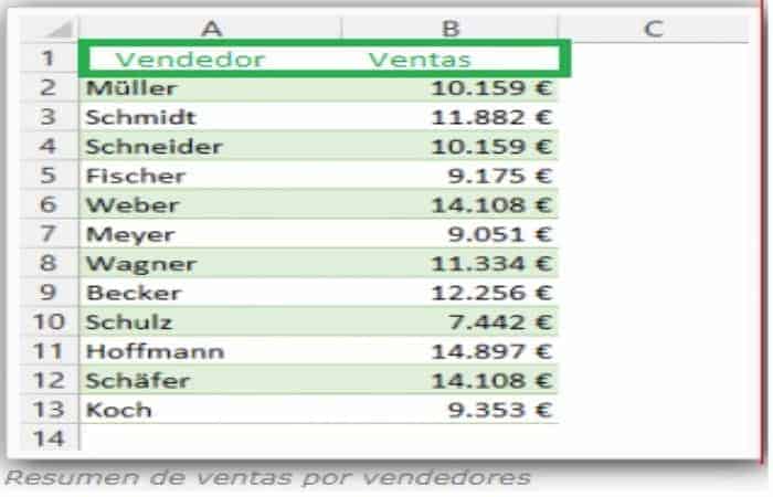
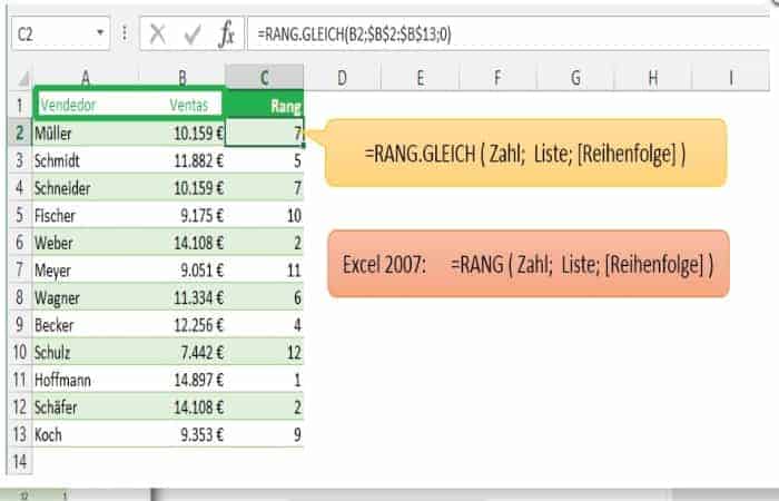
Before creating a ranking table in Excel, it's important to understand how each item is ranked in your list. Let's say you have a sales list with many salespeople and you want to know who the top 5 are. This is where the RANK EQ or RANK function comes in . A ranking table would look like this:

Steps to organize the elements

Giving an order to the elements is very useful so that you do not get confused when analyzing or studying the data that the Excel position table will give you, whether you are organizing statistical information, special data about a survey or related to the sports world, among others.

• Step 1:   Mark the cell with the information.
• Step 2:  Choose with the mouse Home > Sort and filter.
• Step 3:  Mark where it says: Order from A to F (depending on the number of elements).
• Step 4:  Arrange the selected column in ascending order, or click Sort F to A to sort the items in the selected column in descending order.

Example for determining the order of elements when creating a position table in Excel

Let's say you have a company or business and you want to create a table in Excel to analyze it and find out who the best salesperson is so you can meet with all the employees to change their sales strategies, as well as the most outstanding ones. First you must know that the EQ RANK function is used to determine the respective rank of the individual salesperson and depending on the values ​​you enter, the ranks will be ordered. In this case, as seen in the table, the value 0 was left out and the largest element in the list receives the rank 1, so it is ordered in descending order.

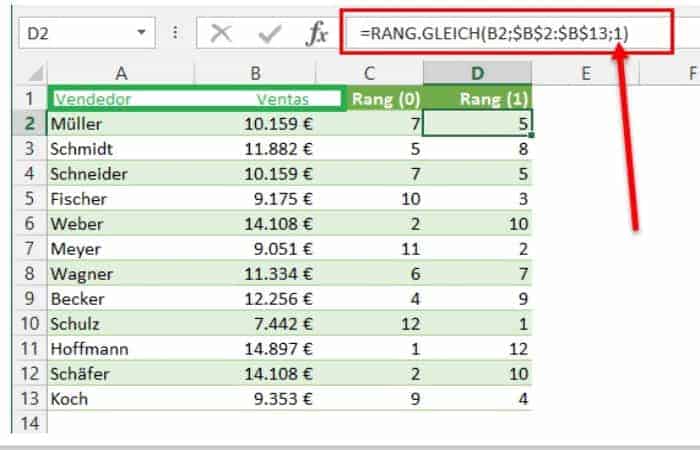
If you use the value 1 as the order instead, the rank is determined ascendingly, that is, the smallest value in the list gets rank 1.

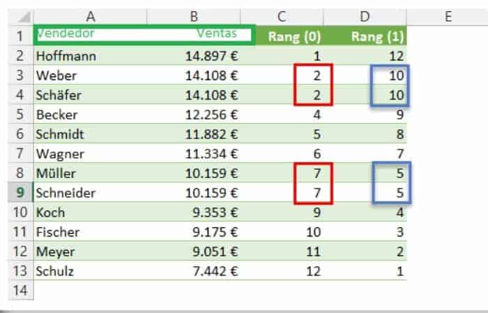
If you now sort the sales list and several values ​​have the same rank, the next one is skipped for the other value. In our example, there are two rank 2s and two rank 7s, so ranks 3 and 8 are not assigned.

Precautions on using tables in Excel

Many experts advise against creating a password table in Excel. Individual secret data can be easily listed and thus quickly at hand, but not adequately protected against unauthorized access. Even beginners can easily bypass the program's password protection and then gain direct access to your data. So be very careful!

You should know that position tables in Excel are not the only option you have to work and study your data, you can also make a dynamic table which is a summary of information generated from a previous table or content base of greater proportion from existing data, although it is rarely used because many people do not really know that it is possible.

You might also be interested in reading about: How to Highlight Active Rows in Excel

To create a pivot table, simply click on any cell and then click on " Table " in the "Insert" tab. You can then change the pivot table to one of the predefined color swatches in the design, or you can choose your own color swatch by clicking on the table, then on the "Table Tools" tab, and finally on "Design" in the table formatting templates.

Finally, it is important to keep in mind when creating your ranking table in Excel that with the RANK and EQUAL RANK functions, Microsoft can create infinite lists. To obtain satisfactory results in your analysis, remember to order the table according to the importance of the data.