How to Use the QUARTILE Function in Excel – Complete Guide

La quartile function in excel helps to return the quartile of a data set in Excel. Going further in this tutorial, you will see How to Find Quartile Using ExcelYou will notice that quartiles are used several times in sales and also when inspecting sample data.

La quartile function in excel It will help you divide the population into groups. For instance, let us consider an example, you can even use the QUARTILE function in Excel to find out the income of a population, i.e. the top 25 percent of income of a population.

La Excel QUARTILE function helps to return the quartile, individually out of the four equal groups. This is for a data set. The QUARTILE function will help to return the minimum value, first quartile, second quartile, third quartile and then the maximum value.

You may be interested in reading about: How to Hide Rows Based on Cell Value in Excel (2 Easy Methods)

Purpose of the Excel QUARTILE function

The purpose of using the Excel QUARTILE function  is to present a set of data.

• Return value: You need to know the requested value for the quartile
• Syntax: =QUARTILE (array, quarter)

Arguments:

• matrix: a reference containing the data to be analyzed.
• quarter: the quartile value to return.

Here we will learn how to use quartile function, highlight quartile, use multiple quartile function and percentile function in dashboard course.

What is Quartile in Excel?

Quartile Function in Excel. The Quartile function is a type of quantile (in statistics). The three points that will divide the sorted data sets into four groups (the groups are equal). Each of them represents one-fourth of the distributed sample population.

There are three quartiles as you talk about the quartile function:

• The first quartile also called (Q1)
• The second quartile also called (Q2)
• The third quartile also called (Q3)

How to use the quartile function in Excel

To use the quartile function in Excel, you need to follow the steps below,

1. The quartile function in Excel returns the quartile (each of four equal groups) for a given set of data.
2. Obtaining a quartile function on a data set
3. Value returned for the requested quartile
4. Use syntax = QUARTILE (matrix, quarter)
   array: a reference containing data to be analyzed
   fourth: the return value of the quartile
5. Use the QUARTILE function to obtain the quartile of a given data set.

Practice notes:

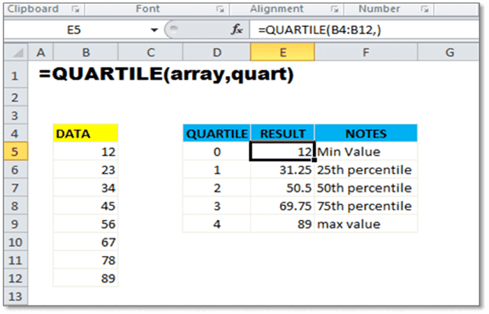
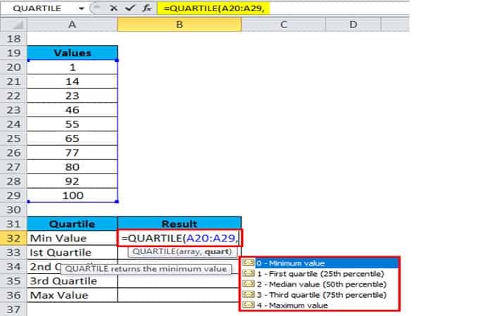
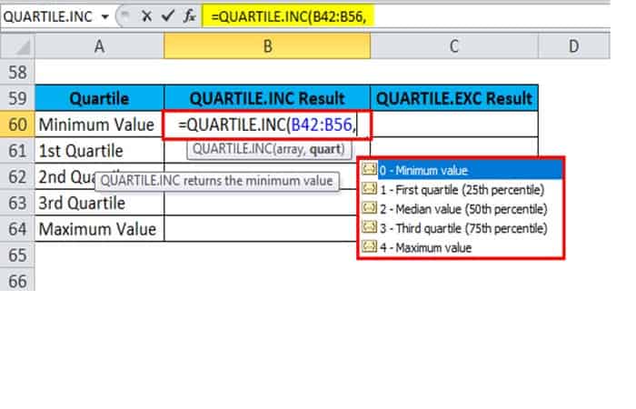
La QUARTILE function in Excel will be used for a set of data to get the quartile. QUARTILE contains two arguments, the array and the quartile. The array contains the numeric data that will help you analyze and the quartile that tells what quartile value will be returned. 5 values ​​are shown for the quartile argument. Here you can see how the QUARTILE function accepts these values.

IMPORTANT: The Quartile Function has been replaced by one or more new Functions. These Functions propose higher accuracy in the results. And the names of these already reflect their use. The Quartile Function is available till date. But this used to be useful for backward compatibility. Since there might not be availability of the Quartile Function in the future. Therefore, people should not rely on these Functions anymore.

How to Find the Quartile Function in Excel

To find the quartiles of this data set in Excel, follow these steps:

1. Step 1:: Follow the order of the data from smallest to largest
2. Step 2:: Divide the data set into two halves after finding out the median
3. Step 3:: Now find the median of the two halves.

Percentiles and quartiles in Excel are easy and therefore should be known by everyone.

Examples of QUARTILE in Excel

Quartile denotes 4 equal portions of the same group or population. In Excel, with the help of the function Quartile, we can find at what extent the portion of the group will start. For example, if in a group of 4 numbers it starts from 1 to 4, if you want to know at what point the 2nd quarter or portion will start. This would be a quartile value of the selected population.

Uses of the QUARTILE function:

The QUARTILE function in Excel returns the quartile for a given set of data. This function divides the data set into four equal groups. QUARTILE will return the minimum value, the first quartile, the second quartile, the third quartile, and the maximum value.

The QUARTILE function in Excel is a built-in function and belongs to the category of statistical functions. This function is also known as a worksheet function in Excel. As a worksheet function, this function can be used as a part of the formula in a cell of a worksheet.

QUARTILE Formula in Excel:

Below is the QUARTILE formula in Excel:

Where the supplied arguments are:

• Matrix: is the array or range of cells of numerical values ​​for which we want the quartile value.
• Fourth: the quartile value to be returned.

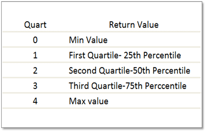
The Quartile function in Excel accepts 5 values ​​as a quarter (second argument), which is shown in the following table:

QUART value	Return value
0	Minimum event value
1	First quartile – 25th percentile
2	Second Quartile – 50th percentile
3	Third Quartile – 75th percentile
4	Maximum event value

As a worksheet function in Excel, the QUARTILE function can be used as part of a formula like the following:

Where is the QUARTILE function located in Excel?

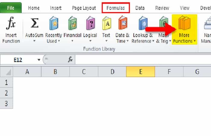
The QUARTILE function is a built-in function in Excel; therefore, it is located in the FORMULAS tab. Follow the steps below:

1. Step 1:: Click on the FORMULAS tab. Click on the More functions option.

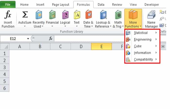
2. Step 2:: A drop-down list of feature categories will open.

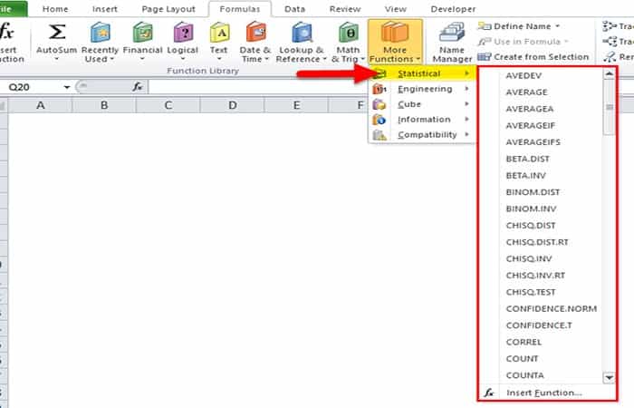
3. Step 3:: Click on the category Statistical functionsA drop-down list of functions will open.

4. Step 4:: Select the QUARTILE function from the drop-down list.

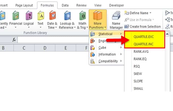
NOTE: : In the above screenshot, as we can see, there are two functions listed with the name QUARTILE:

1. QUARTILE.EXC
2. QUARTILE.INC

In the new version of Excel, the QUARTILE function has been replaced by these two functions, giving more precision in the result. However, in Excel, the QUARTILE function is still available, but it could be replaced in the future by these functions at any time.

How to use the QUARTILE function in Excel?

The QUARTILE function is very simple to use. Let us now see how to use the TILE function in Excel with the help of some examples.

Example 1

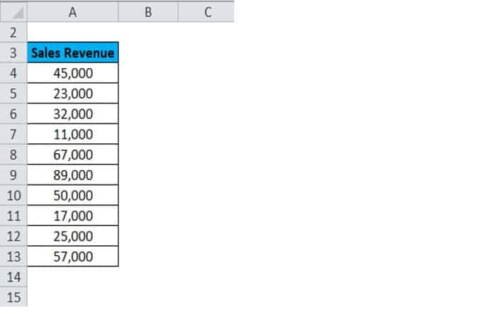
We have given some sales figures:

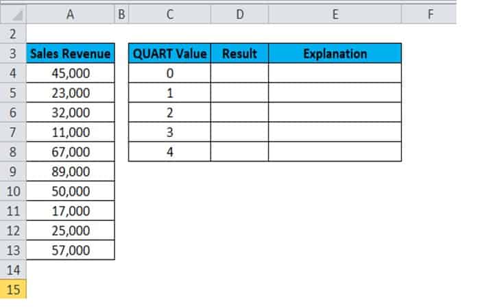
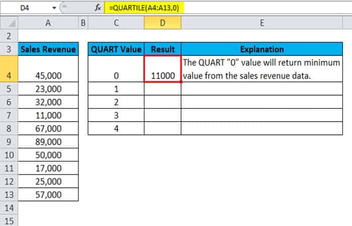
Here, we will calculate the minimum value, first quartile, second quartile, third quartile, and maximum value using the QUARTILE function. We will take the value of the second QUARTILE argument from 0-4 of the QUARTILE function as shown in the following screenshot for this calculation.

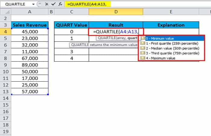
Now we will apply the QUARTILE function to the sales data.

We will calculate the QUARTILE function for all values ​​one by one by selecting values ​​from a drop-down list.

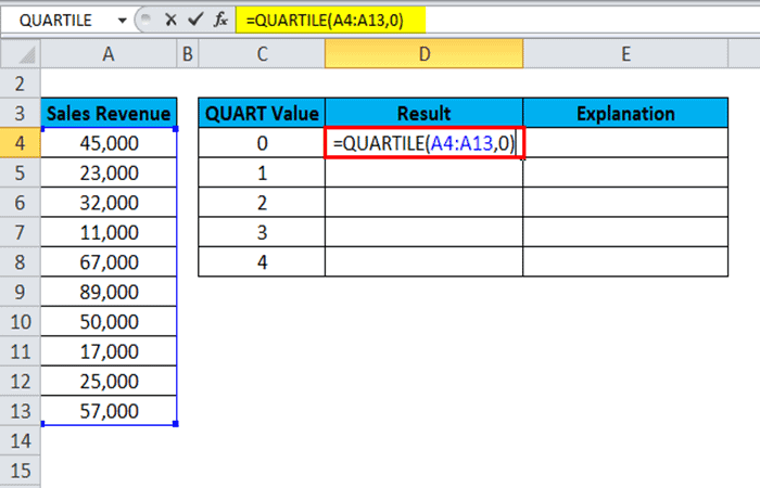
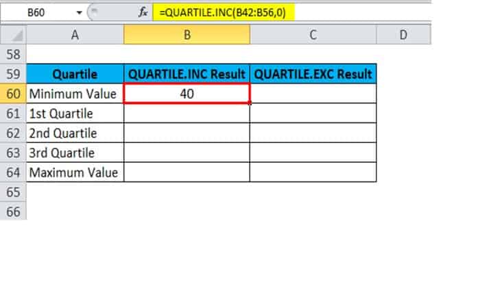
The result is:

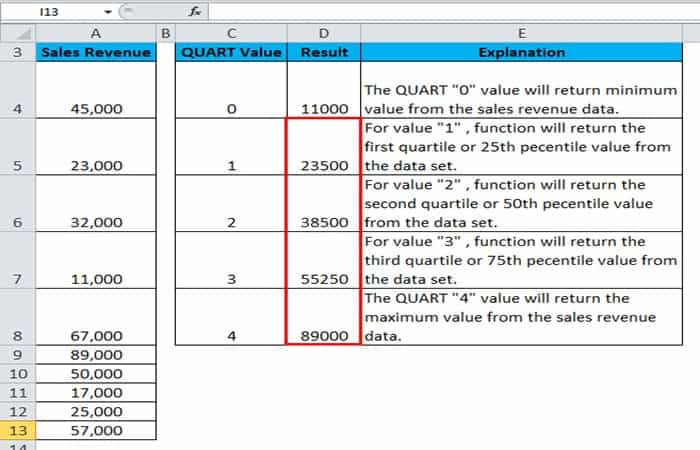
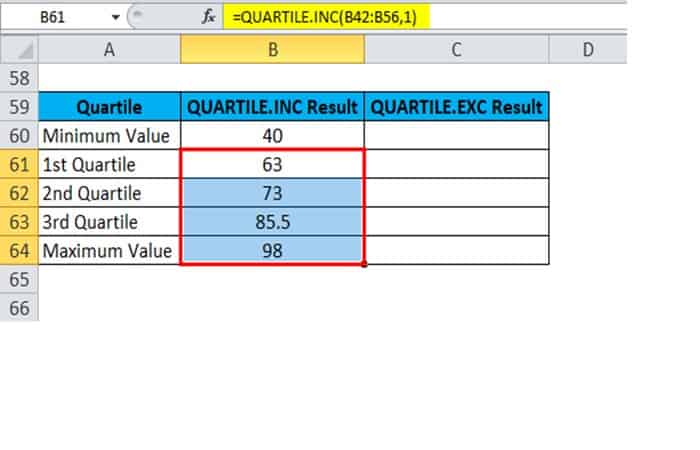
Similarly, we will find other values. The final result is shown below:

Explanation:

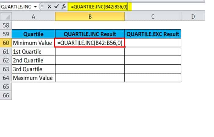
• We pass the array or cell range of data values ​​for which you need to calculate the QUARTILE function.
• We pass the value 0 as the second argument to calculate the minimum value of the given data set.
• We enter the value 1 for the first quartile.
• We enter the value 2 for the second quartile.
• We enter the value 3 for the third quartile.
• We introduce the value 4 as the second argument, which will give the maximum value in the data set.

Example 2

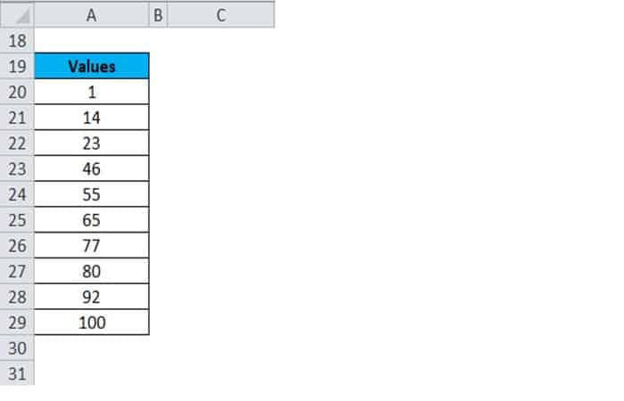
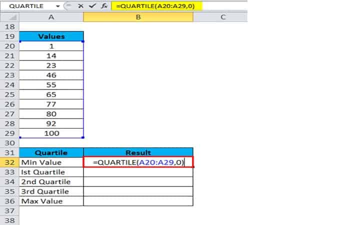
Let us take another dataset where the data is arranged in ascending order to better understand the usage of Excel's QUARTILE function:

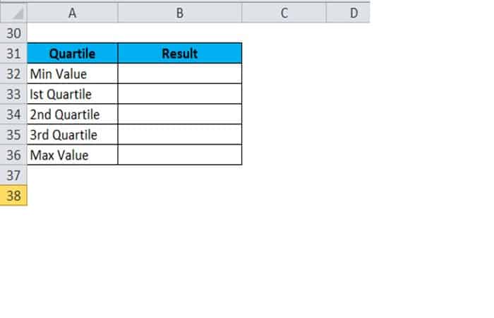
1. Step 1:: Now we will calculate the following quartile values:

The formula is shown below:

2. Step 2:: We will calculate the QUARTILE function for all the values ​​one by one by selecting the values ​​from a drop-down list.

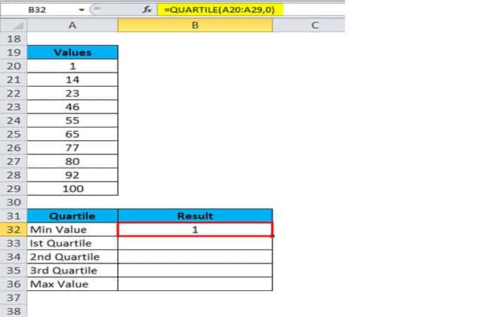
The result is:

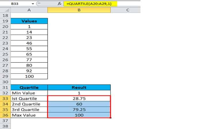
Similarly, we will find other values. The final result is shown below:

Explanation:

• If we look at the result closely, 1 is the minimum value of the given data set.
• 100 is the maximum value in the data set.
• The value of the first quartile is 28,75, the value of the second quartile is 60, and the value of the third quartile is 79,25.
• The QUARTILE function divides the data set into 4 equal parts. This means that we can say that 25% of the values ​​lie between a minimum value and 1st
• 25% of the values ​​are between 1st and 2nd
• 25% of the values ​​are between 2nd and 3rd
• The 25% values ​​are among the 3rd ^y the maximum value.

Now we will study the use of the QUARTILE EXC and QUARTILE INC functions since in the future the QUARTILE function in Excel can be replaced by these functions.

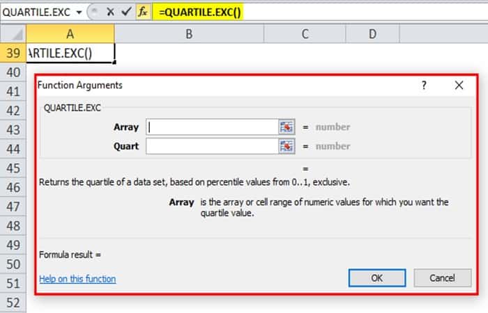
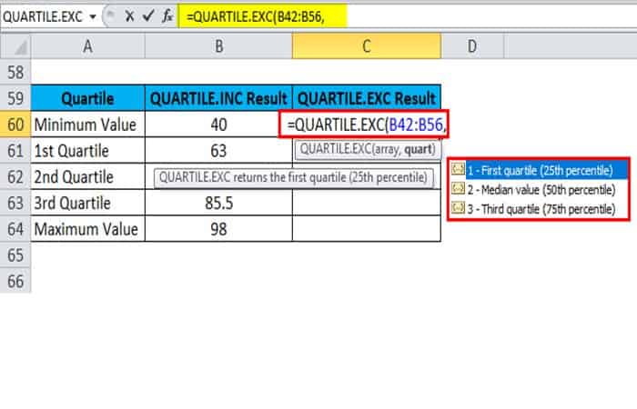
The SYNTAX of QUARTILE EXC and QUARTILE INC is the same. If we choose the QUARTILE EXC function from the function drop-down list in the Statistical Functions category, a dialog box for the function arguments will open.

The arguments for PASS are the same as the QUARTILE function in Excel.

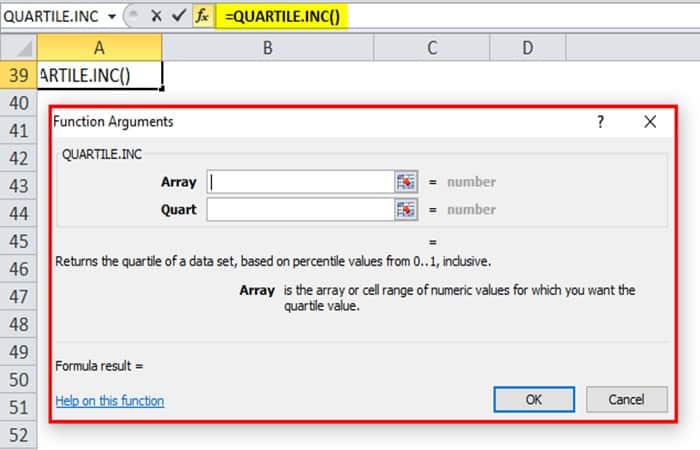
If we select the INC QUARTILE function, it will also open a dialog box for the function arguments as shown below:

• NOTE: : The QUARTILE INC function returns the quartile of a data set, based on percentile values ​​from 0 to 1, inclusive. While the QUARTILE EXC function returns the quartile of a data set, based on percentile values ​​from 0 to 1, exclusive.

Now, in the following examples, we will see the difference between the above two functions.

Example 3

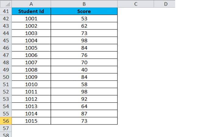
Let's assume the test scores below for a class.

We will apply the QUARTILE EXC and QUARTILE INC functions on the above scores and closely observe the result of these functions.

1. Step 1:: First, we are calculating the INC QUARTILE function. We pass the list of scores as the first argument to the function and choose the second argument from the list 0-4 for the minimum values, 1 ^°, 2 ^° , 3 ^° and maximum, one by one, as shown below:

2. Step 2:: We will calculate the QUARTILE function for all the values ​​one by one by selecting the values ​​from a drop-down list.

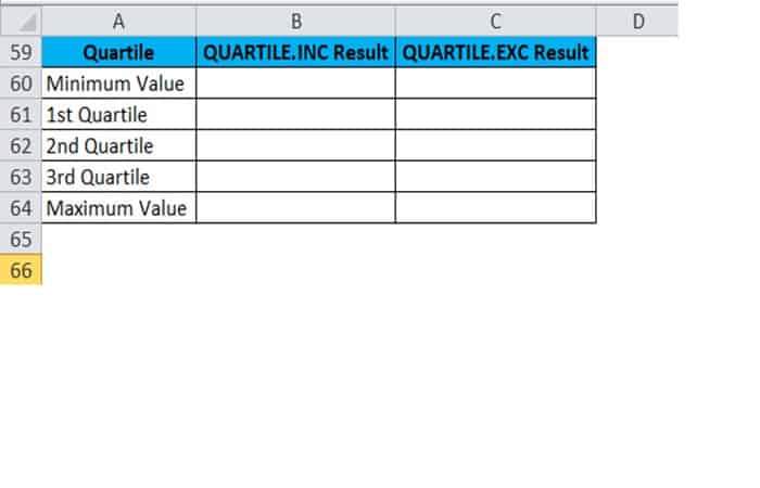
The result is:

Similarly, we will find other values. The final result is shown below:

The same steps will be followed to calculate the EXC QUARTILE function.

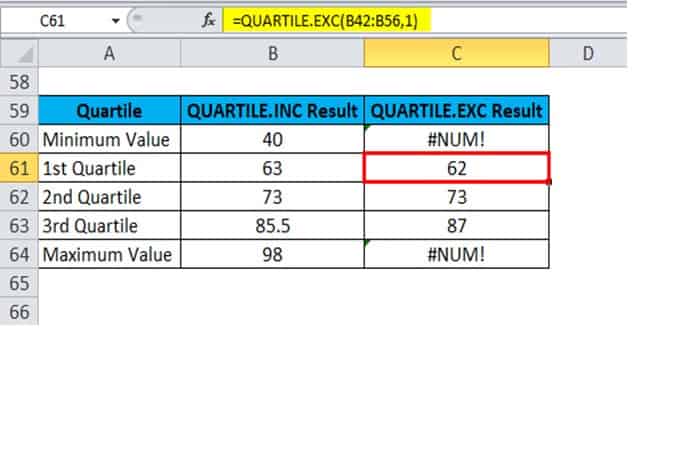
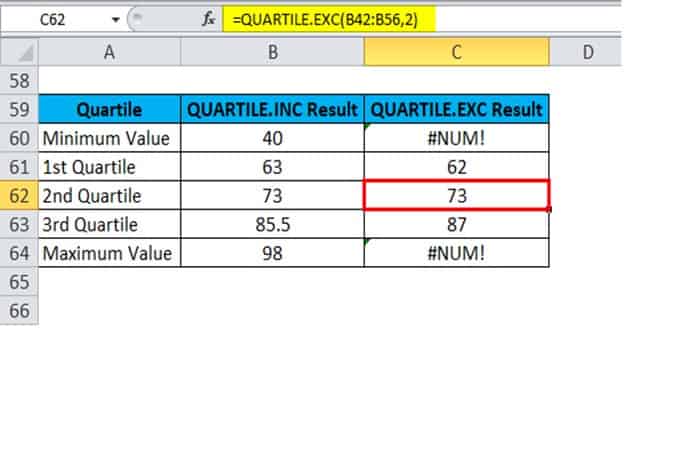
QUARTILE.EXC Function 1st, 2nd, and 3rd quartile values.

The results are:

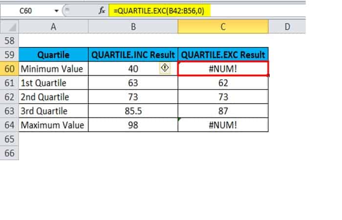
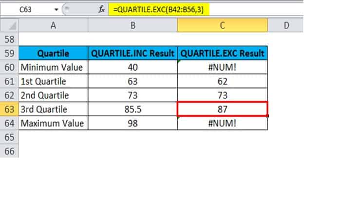
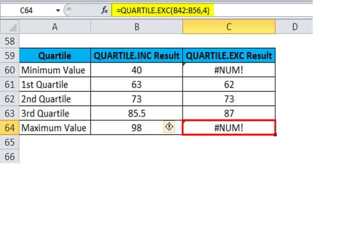
Explanation:

• Suppose you see the above results for values ​​0 and 4, the QUARTILE EXC function returns the #NUM! an error value because it calculates only the 1st, 2nd, and 3rd quartile values. Whereas the QUARTILE INC function works the same as the QUARTILE function.
• The value of the second quartile is the same for both functions.
• The value of the first quartile of EXC QUARTILE will be slightly lower than the INC QUARTILE.
• The value of the third quartile of QUARTILE EXC will be slightly higher than QUARTILE.INC.

MS Excel: How to use the QUARTILE (WS) function

In this part of the Excel tutorial we will explain how to use the QUARTILE function in Excel with syntax and examples.

Description

The QUARTILE function in Microsoft Excel returns the quartile of a set of values. The QUARTILE function in Excel is a built-in function that is classified as a statistical function. It can be used as a worksheet (WS) function in Excel. As a worksheet function, the QUARTILE function can be entered as part of a formula in a cell of a worksheet.

Syntax

The syntax for the QUARTILE function in Microsoft Excel is: QUARTILE (array, nth_quartile)

Parameters or Arguments

Formation: A range or array from which you want to get the nth quartile.

nth_quartile: The quartile value you want to return. This can be one of the following values:

Price	Explanation
0	Smallest value in the data set
1	First quartile (25th percentile)
2	Second quartile (50th percentile)
3	Third quartile (75th percentile)
4	Largest value in the data set

Returns: The QUARTILE function returns a numeric value.

Example (as a worksheet function)

Let's look at some examples of the Excel QUARTILE function and explore how to use the QUARTILE function as a worksheet function in Microsoft Excel:

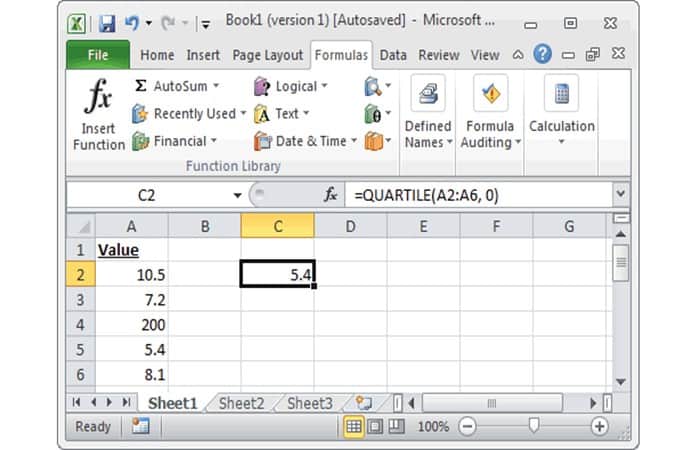
According to the Excel spreadsheet above, the following QUARTILE examples would return:

=QUARTILE(A2:A6, 0)Result: 5.4 =QUARTILE(A2:A6, 1)Result: 7.2 =QUARTILE(A2:A6, 2)Result: 8.1 =QUARTILE(A2:A6, 3)Result: 10.5 =QUARTILE(A2:A6, 4)Result: 200 =QUARTILE({7,8,9,10}, 0)Result: 7 =QUARTILE({7,8,9,10}, 1)Result: 7.75 =QUARTILE({7,8,9,10}, 2)Result: 8.5 =QUARTILE({7,8,9,10}, 3)Result: 9.25 =QUARTILE({7,8,9,10}, 4)Result: 10

How to calculate a quartile in Excel

This part of the article introduces quartiles and the different methods for calculating them in Excel. You will find an overview of quartiles, how they work, and how to calculate them.

Quartiles are widely used in statistics, they allow to divide a selected group. Below is a more detailed description with an example. Quartiles can be used in Geomarketing.

This allows the data to be divided into several groups, which can then be represented in the form of classes. It will be enough to use software to represent this on a map, for example, or in the form of a graph.

What are quartiles?

Quartiles represent the boundaries between groups in a selection. In our case, the data file contains 96 departments, each with associated data (taxes per inhabitant), the quartiles will separate my departments into several groups.

• E.g., the 1st quartile will show me the 24 departments (96/4, so 25%) with the lowest per capita taxes, the 2nd quartile (representing the median, so 50%) will indicate the 48 departments with the lowest taxes per inhabitant, and you will have understood that the 3rd quartile will show me the 72 departments (therefore 75%) with the lowest taxes.

We can reverse the logic, for example for the 3rd quartile which tells me the 72 departments with the lowest taxes, the rest of the departments therefore correspond to the 24 departments with the highest taxes. In Excel, you can see the extreme quartiles, the 0th and 4th quartiles, the first being the lowest value in the selected data range and the second being the highest.

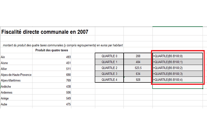
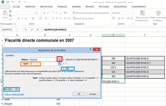
Method 1: Direct calculation of a quartile in Excel

The first method illustrated by the screenshot below allows you to calculate the quartiles directly in the cells by inserting the appropriate formula.

• For example, to calculate the first quartile, we use the formula:
  • =QUARTILE(your_range:of_data;1).

The result of the first quartile is 484. Therefore, in 25% of the departments the taxes are less than 484 euros per inhabitant.

«your_data_range» You can select it directly using the mouse or you can enter your data range (B5:B100 in the example).

You can see that to the right of my data range there is a semicolon followed by the number 1. You need to replace this number with the quartile you want to appear, in the screenshot below you can see the different possibilities.

Method 2: Calculate a Quartile in Excel Using the Function Icon

This second method uses icon functions to calculate quartiles.

1. Step 1:: First, you need to select the cell where you want your quartile to appear.
2. Step 2:: Once selected, click on the functions icon, in the “Find a function» (first black rectangle) enter the quartile, then select the appropriate function that appears just below (second black rectangle).

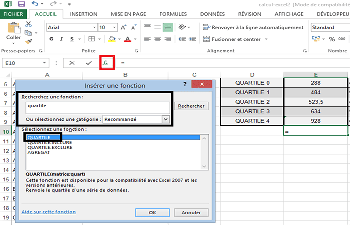
NOTE: : A new window opens. In the matrix, click the icon on the right (red rectangle in the screenshot below) to select your data range.

3. Step 3:: In Quart (orange rectangle), indicate which quartile you want to obtain (0 – 1 – 2 – 3 – 4). The result display appears (blue rectangle), you can validate so that it appears in the selected cell upstream.

You may also be interested in reading about: How to Use Regular Expressions in Excel – Complete Guide

Conclusion

As you can see, we have just learned how to calculate and use the quartile function in Excel, but you may want to discover other types of calculations possible with the software. In fact, it offers incredible possibilities that will allow you to manage your various activities. We hope we have helped you with this information.