How to Hide Rows in Excel Easily. 3 Easy Methods

In this article, we'll show you how to hide rows in Excel . Working with large datasets containing row upon row of data can be quite challenging. In such cases, finding data that matches specific criteria can feel like searching for a needle in a haystack. Fortunately, Excel provides features that allow you to hide certain rows based on cell values, so you only see the rows you want. There are several ways to do this. We'll explore various methods, and you can choose the one that best suits your needs.

You might also be interested in: Emojis in Excel: 4 Ways to Insert Them and How to Use Them

How to hide columns and rows in Excel easily

There are several ways to hide and show columns and rows in Excel. One thing you might not know: you can hide and show more than one column or row at the same time , even if they aren't adjacent. Even better, if they are adjacent, you can use Excel's Grouping tool . Below, we describe a couple of ways to hide and show your Excel columns and rows to save you time.

Hide and show columns and rows

These are the steps you must follow:

• Step 1: Select the number of columns or rows you want to hide (use the key Control to select additional discontiguous columns or rows).
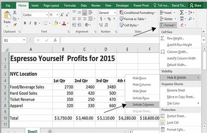
• Step 2: click the button Format located in the tab Home / Cells group and then choose Hide columns or rows (another option is to right-click on a highlighted column or row header and select hide).
• Step 3: Your columns and rows are now hidden.

Show all columns or rows

In this case you must do the following:

• Step 1: Click the Format button located under the tab Home / Cells group, then choose Show columns or rows (Another option is to drag over the range of columns or rows you are interested in displaying. Then right-click on the column or row header and choose unhide.)
• Step 2: Your columns and rows are now visible.

Hide and show columns and rows using the group function

The following steps describe how to use the Group option in Excel for versions 2007, 2010, 2013, and 2016. Grouping only works with adjacent columns and rows. Here are the steps you should follow:

• Step 1: Select the number of contiguous rows or columns you want to hide (you cannot use the key Control during this operation).
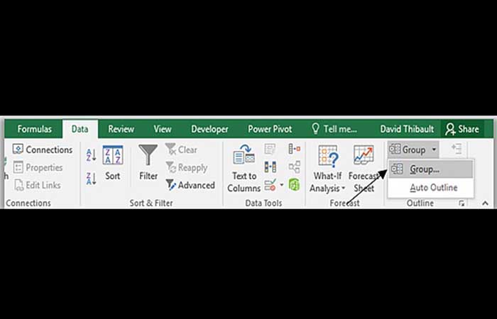
• Step 2: click the button Group located in the tab Data / Schema group and then choose.

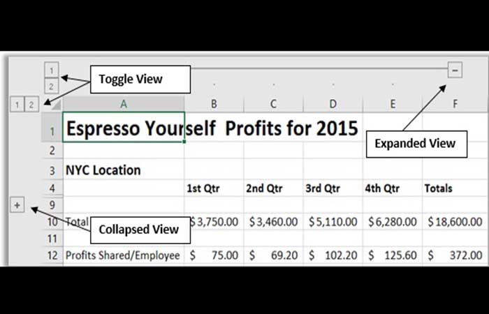
• Step 3: Your columns and rows are now hidden. Not only are your columns or rows hidden, but Excel has added show and hide buttons to help you toggle your view:

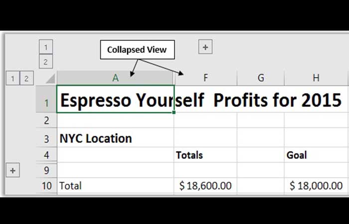
Collapsed view of columns:

To disable the group function

In this case, the procedure is as follows:

• Step 1: select the rango of columns or rows that you would like to ungroup.
• Step 2: click the button Group located in the tab Data / group, Scheme and then choose.
• Step 3: The Grouping feature is now removed.

Using Filters to Hide Rows in Excel Based on Cell Value

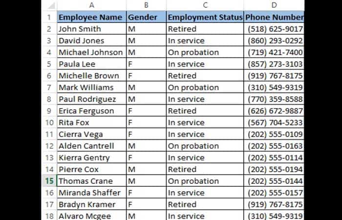
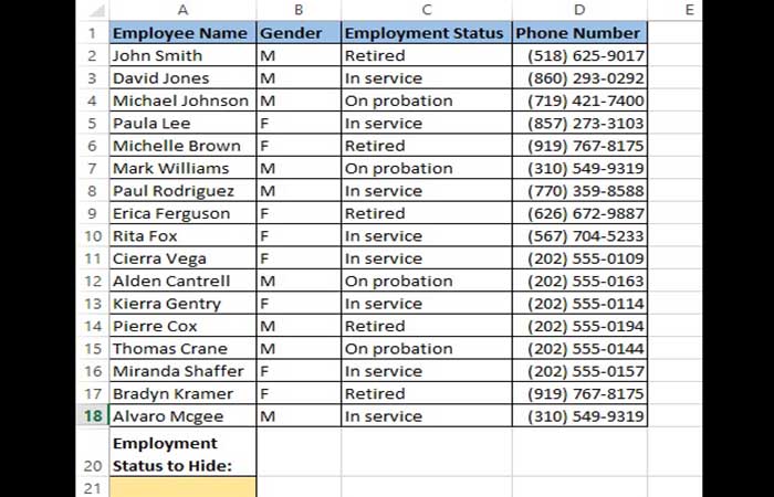
Suppose you have the dataset shown below and you want to see data only about employees who are still In service.

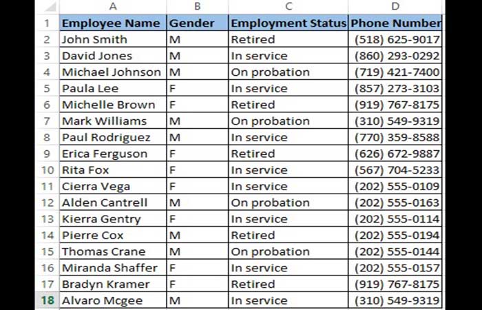
This is really easy to do using filters. Here are the steps you need to follow:

Step 1: Select the work area of ​​your dataset.

Step 2: On the Data tab , select the Filter button . You'll find it in the 'Sort & Filter ' group.

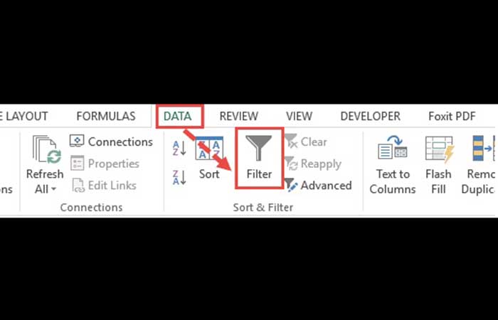
Step 3: You should now see a small arrow button in each cell of the header row.

Imagen8

Step 4: These buttons are designed to help you filter your cells. You can click any arrow to choose a filter for the corresponding column.

Step 5: In this example, we want to filter the rows that contain the employment status = "In service". Therefore, select the arrow next to the Employment Status heading.

Step 6: Uncheck the boxes next to all statuses except " In service ". You can simply uncheck " Select all " to quickly uncheck everything and then select " In service ".

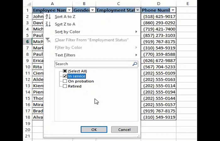
Step 7: Click OK.

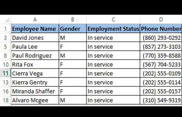
You should now only be able to see the rows with Employment Status = " In service ". All other rows should now be hidden.

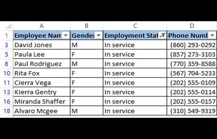
Note: To show hidden cells, simply click the Filter button again.

Using VBA to Hide Rows in Excel Based on Cell Value

The second method requires a bit of coding. If you are used to using macros and a bit of coding using VBA, then you get a lot more scope and flexibility to manipulate your data to behave exactly the way you want.

Writing VBA code

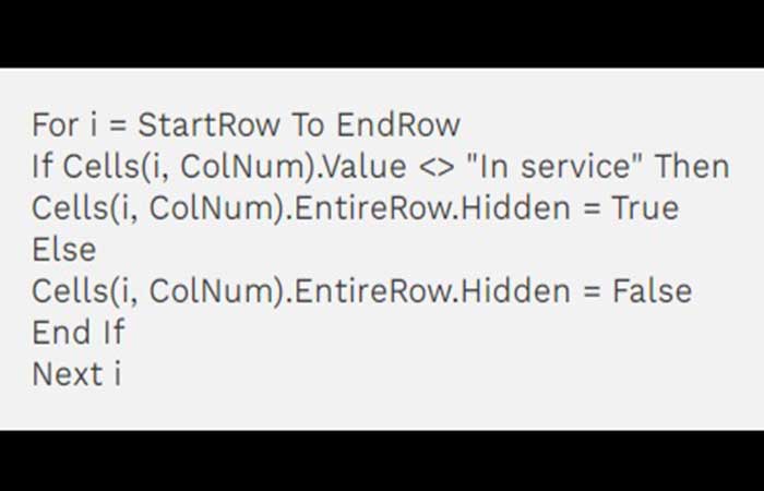
The following code will help you to display only the rows that contain information about employees who are 'In service' and hide all other rows:

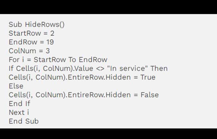
The macro iterates through each cell in column C and hides the rows that do not contain the value "In service". Essentially, you need to analyze each cell in rows 2 through 19 and set the ' Hidden ' attribute of the row you want to hide. To enter the code above, copy and paste it into your developer tools window. Here's how:

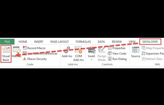
Step 1: On the Developer menu ribbon , select Visual Basic.

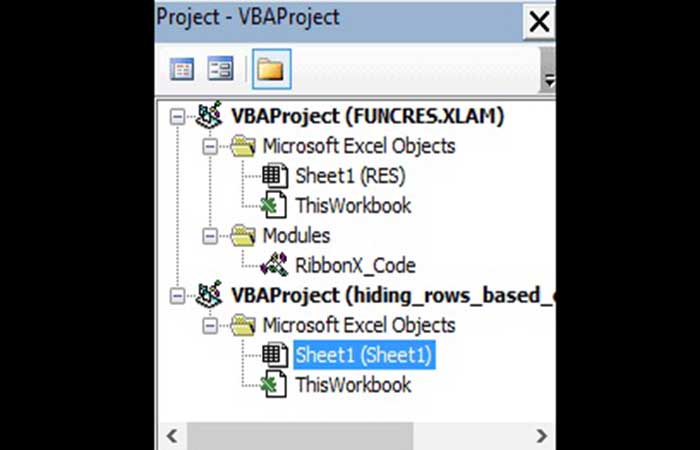
Step 2: Once the VBA window opens, you'll see all your files and folders in the Project Explorer on the left. If you don't see the Project Explorer, click View -> Project Explorer.

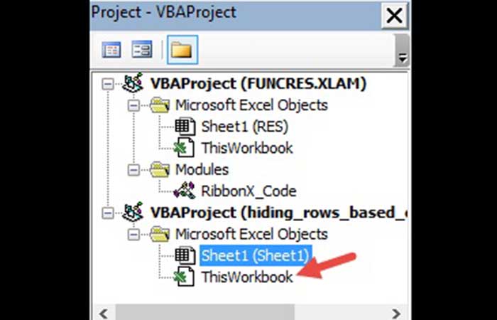
Step 3: Make sure ' ThisWorkbook ' is selected in the VBA project with the same name as your Excel workbook.

Step 4: Click Insert-> Module . You should see a new module window open.

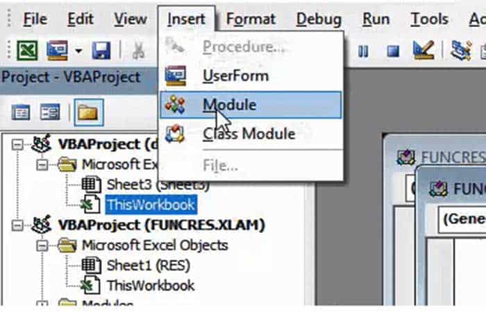
Step 5: Now you can start coding. Copy the lines of code above and paste them into the new module window.

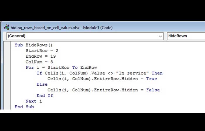
Step 6: In our example, we want to hide the rows that do not contain the value 'In service' in column 3. But you can replace the ColNum value of “3” in line 4 with the column number that contains the criteria values.

Step 7: Close the VBA window.

Note: If your dataset covers more than 19 rows, you can change the values ​​of the StartRow and EndRow variables to your required row numbers.

If you don't see the Developer option, go to Options in the File menu . Select Customize Ribbon and check the Developer option under Main Tabs.

Step 8: Finally, click OK.

Your macro is now ready to use.

You might also want to know: How to Export from Microsoft Project to Excel

Running the macro

Whenever you need to use the above macro, all you need to do is run it, and here's how:

Step 1: Select the Developer tab.

Step 2: Click the Macros button (in the Code group).

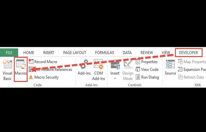
Step 3: This will open the Macros Window, where you will find the names of all the macros you have created so far.

Step 4: Select the macro (or module) called ' HideRows ' and click the Run button.

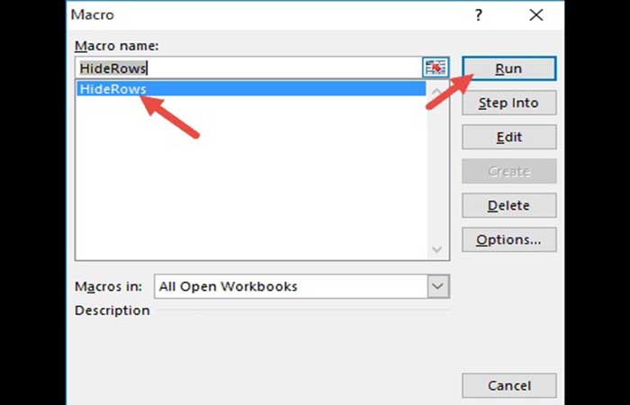
You should see all the rows where the Employment Status is not Hidden as " In servic e".

Explanation of the Code

Here is a line-by-line explanation of the above code:

In line 1 we define the name of the function.

Sub HideRows ()

In lines 2, 3, and 4 we define variables to hold the start row and the end row of the dataset, as well as the index of the criteria column.

StartRow = 2

EndRow = 19

ColNum = 3

In lines 5 through 11, we iterated through each cell in column “3” (or column C) of the active worksheet. If a cell does not contain the value “In service”, then we set the 'Hidden' attribute of the entire row (corresponding to that cell) to True, which means we want to hide the entire corresponding row.

Line 12 simply delimits the end of the HideRows function.

End Sub

In this way, the code above hides all rows that do not contain the value ' In service' in column C.

Display columns based on cell value

Now that we have been able to hide rows in Excel that are not needed, what if we want to see the hidden rows again? Doing this is pretty easy. You just need to make a small change to the HideRows function.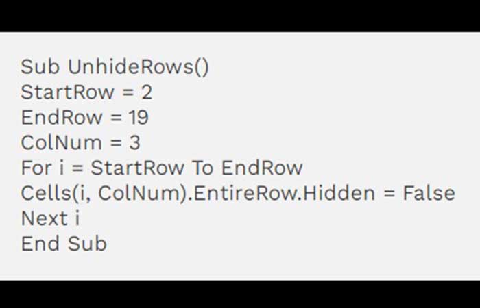

Here, we simply make sure that regardless of the value, all rows are shown (by setting the Hidden property of all rows to False). You can run this macro in exactly the same way as HideRows.

Hide rows based on cell values ​​in real time

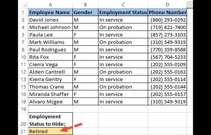
In the first example, the columns are hidden only when the macro is running. However, most of the time, we want to hide columns on the fly, based on the value of a particular cell. So, now let's take a look at another example that demonstrates this. In this example, we have the following dataset:

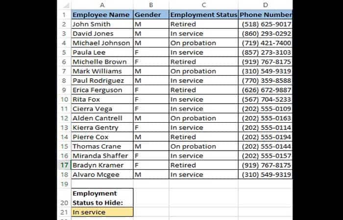
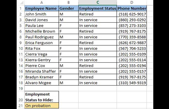
The only difference from the first dataset is that we have a value in cell A21 that will determine which rows should be hidden. So, when cell A21 contains the value 'Retired', only the rows containing the employment status 'Retired' are hidden. Similarly, when cell A21 contains the value 'On probation' , only the rows containing the employment status 'On probation' are hidden.

When there is nothing in cell A21, we want all the rows to be displayed. We want this to happen in real time, every time the value in cell A21 changes. To do this, we need to use Excel's Worksheet_SelectionChange function.

The Worksheet_SelectionChange event

The Worksheet_SelectionChange procedure is a built-in VBA event in Excel . It comes pre-installed with the worksheet and is triggered whenever a user selects a cell and then changes their selection to another cell.

Since this function comes pre-installed with the worksheet, you must place it in the correct worksheet code module in order to use it. In our code, we are going to put all our lines inside this function, so that they are executed every time the user changes the value in A21 and then selects some other cell.

Writing VBA code

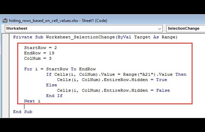
Here is the code we are going to use:

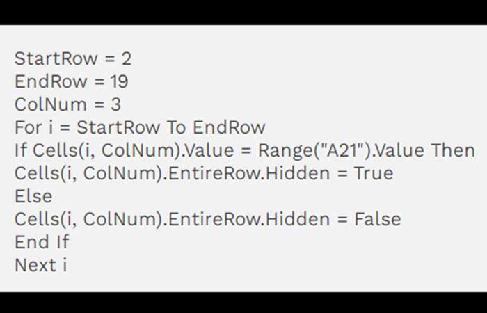
To enter the code above, you must copy and paste it into your developer window, within the Worksheet_SelectionChange procedure of your worksheet. Here's how:

Step 1: On the Developer menu , select Visual Basic.

Step 2: Once the VBA window opens, you will see all the files and folders of your project in the Project Explorer on the left side.

Step 3: In the Project Explorer, double-click the name of your worksheet, located under the VBA project with the same name as your Excel workbook. In our example, we are working with Sheet1.

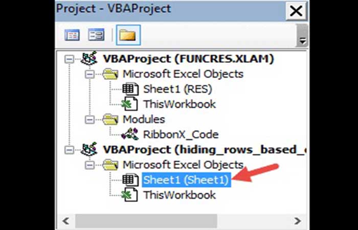
Step 4: This will open a new module window for the selected sheet.

Step 5: Click the drop-down arrow on the left side of the window. You should see an option that says " Worksheet ".

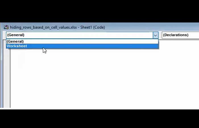
Step 6: Click on the 'Worksheet' option . By default, you will see the Worksheet_SelectionChange procedure created for you in the module window.

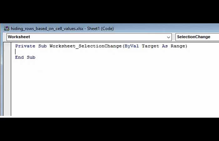
Step 7: Now you can start coding. Copy the lines of code above and paste them into the Worksheet_SelectionChange procedure, right after the line: Private Sub Worksheet_SelectionChange (ByVal Target As Range).

Step 8: Close the VBA window.

Running the macro

The Worksheet_SelectionChange procedure starts running as soon as you finish coding. Therefore, you don't need to explicitly run the macro for it to start working. Try typing ' Retired ' in cell A21, then click on any other cell. You should find that all the rows containing the value 'Retired' in column C disappear.

Now try replacing the value in cell A21 with 'On probation' , then click on any other cell. You should find all the rows containing the value 'On probation ' in column C disappear.

Now try deleting the value in cell A21 and leaving it empty. Then click on any other cell. You should find that both rows become visible again.

This means that the code works in real time when changes are made in cell B20.

Explanation of the Code

Let's take a few minutes to understand this code now.

Lines 1, 2, and 3 define variables to hold the start row and end row of the dataset, as well as the index of the criteria column. You can change the values ​​to suit your needs.

StartRow = 2

EndRow = 19

ColNum = 3

Lines 4 through 10 loop through each cell in column “3” (or column C) of the worksheet. If the cell contains the value in cell A21, then we set the ‘Hidden’ attribute of the entire row (corresponding to that cell) to True, meaning we want to hide the entire corresponding row.

Code5

In this way, the above code hides the rows in the dataset based on the value in cell A21. If A21 does not contain any value, the code displays all the rows.

Check out: How to Combine Excel with Word: Importing Data from Excel to Word

Final thoughts

In this tutorial, we showed you how you can use Filters and Excel VBA to hide rows in Excel based on the value of a cell. We also showed you some simple methods to hide columns and rows in Excel. We did this with the help of two simple examples: one that deletes the required rows only when the macro is run explicitly and another that works in real time. We hope that we have succeeded in helping you understand the concept behind the code so that you can customize it and use it for your own purposes.