Excel CHOOSE Function. Formulas and Examples

This tutorial explains the syntax and basic uses of Excel's CHOOSE function and provides some non-trivial examples that demonstrate how to use a CHOOSE formula. It's one of those Excel functions that might not seem useful on its own, but when combined with other functions, it offers a number of incredible benefits. At its most basic level, the CHOOSE function is used to retrieve a value from a list by specifying the position of that value. Later in this tutorial, you'll find several advanced uses that are definitely worth exploring.

Excel CHOOSE Function: Basic Syntax and Uses

The CHOOSE function in Excel is designed to return a value from a list based on a specific position. The function is available in Excel 365, Excel 2019, Excel 2016, Excel 2013, Excel 2010, and Excel 2007.

The syntax of the CHOOSE function is as follows:

CHOOSE (Index_num, value1, [value2],…)

Where:

Index_num (required): The position of the value to be returned. It can be any number between 1 and 254, a cell reference, or another formula.

Value1, Value2, ...: a list of up to 254 values ​​to choose from. Value1 is required; other values ​​are optional. These can be numbers, text values, cell references, formulas, or defined names. Here is an example of a CHOOSE formula in its simplest form:

=CHOOSE(3, «Mike», «Sally», «Amy», «Neal»)

The formula returns " amy " because Index_num is 3 and "Amy" is the third value in the list:

You might also be interested in: How to Use the Left and Right Functions in Excel

Excel CHOOSE Function: 3 Things to Remember!

CHOOSE is a very simple function and you will hardly find it difficult to implement it in your worksheets. If the result returned by your CHOOSE formula is unexpected or is not the result you were looking for, it may be due to the following reasons:

1. The number of values ​​to choose from is limited to 254.
2. Error is returned.
3. If the argument Index_num is a fraction, it is truncated to the lowest whole number.

How to use the CHOOSE function in Excel – formula examples

The following examples show how CHOOSE can extend the capabilities of other Excel functions and provide alternative solutions to some common tasks, even those that many consider infeasible.

CHOOSE in Excel instead of nested IF

One of the most common tasks in Excel is to return different values ​​based on a specific condition. In most cases, this can be done using a classic nested IF statement. But Excel's CHOOSE function can be a quick and easy-to-understand alternative.

Example 1: Return different values ​​depending on the condition

Suppose you have a column of student grades and you want to label the grades based on the following conditions: Outcome and Score.

• Poor: 0 - 50
• Satisfying: 51 - 100
• Okay: 101 - 150
• Excellent: More than 151

One way to do this is to nest some IF formulas inside each other:

=IF(B2>=151, "Excellent", IF(B2>=101, "Good", IF(B2>=51, "Satisfactory", "Poor")))

Another way is to choose a label that corresponds to the condition:

=CHOOSE((B2>0) + (B2>=51) + (B2>=101) + (B2>=151), «Poor», «Satisfactory», «Good», «Excellent»)

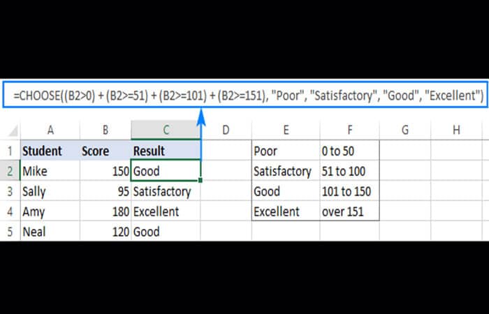
How this formula works:

In the Index_num argument , evaluate each condition and return TRUE if the condition is met, FALSE otherwise. For example, the value in cell B2 meets the first three conditions, so we get this intermediate result:

=CHOOSE(TRUE + TRUE + TRUE + FALSE, "Poor", "Satisfactory", "Good", "Excellent")

Since in most Excel formulas , TRUE equals 1 and FALSE equals 0 , our formula undergoes this transformation:

=CHOOSE(1 + 1 + 1 + 0, "Poor", "Satisfactory", "Good", "Excellent")

Once the addition operation is performed, we have:

=CHOOSE(3, "Poor", "Satisfactory", "Good", "Excellent")

As a result, the 3rd value in the list is returned, which is " good ".

Tips:

• To make the formula more flexible, you can use cell references instead of hard-coded labels, for example:

=CHOOSE((B2>0) + (B2>=51) + (B2>=101) + (B2>=151), $E$1, $E$2, $E$3, $E$4)

• If none of your conditions are TRUE, the argument Index_num will be set to 0, forcing your formula to return the #VALUE! error. To avoid this, simply wrap CHOOSE in the IFERROR function like this:

=IFERROR(CHOOSE((B2>0) + (B2>=51) + (B2>=101) + (B2>=151), «Poor», «Satisfactory», «Good», «Excellent»), «»)

Example 2: Perform different calculations depending on the condition

You can use Excel's CHOOSE function to perform a calculation on a series of possible calculations/formulas without nesting multiple IF statements within each other. As an example, let's calculate each salesperson's commission based on their sales:

• 5% – $0 to $50
• 7% – $51 to $100
• 10% – over $101

With the sales amount in B2, the formula takes the following form:

=CHOOSE((B2>0) + (B2>=51) + (B2>=101), B2*5%, B2*7%, B2*10%)

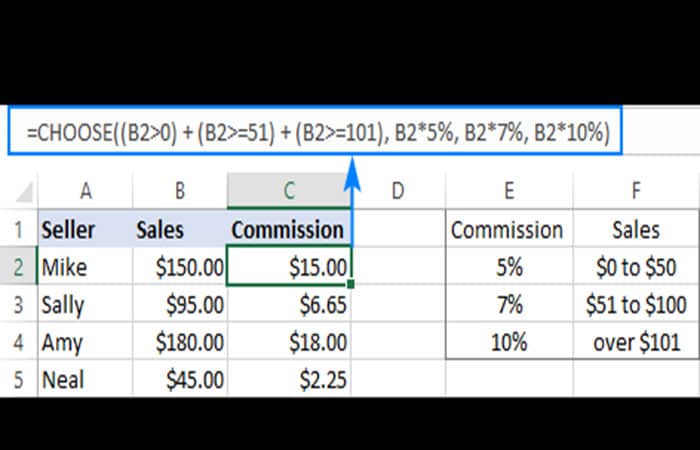
Instead of hard-coding the percentages into the formula, you can refer to the corresponding cell in your reference table, if there is one. Just remember to fix the references using the $ sign.

=CHOOSE((B2>0) + (B2>=51) + (B2>=101), B2*$E$2, B2*$E$3, B2*$E$4)

 The Pick formula to generate random data

As you probably know, Microsoft Excel has a special function for generating random integers between the lower and upper numbers you specify: the RANDBETWEEN function . Use the index_num argument of CHOOSE, and your formula will generate almost any random data you want. For example, this formula can produce a list of random exam results:

=CHOOSE(RANDBETWEEN(1,4), "Poor", "Satisfactory", "Good", "Excellent")

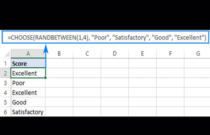
The logic of the formula is obvious: RANDBETWEEN generates random numbers from 1 to 4 and CHOOSE returns a corresponding value from the predefined list of four values.

Note: RANDBETWEEN is a volatile function and recalculates with every change you make to the worksheet. As a result, your list of random values ​​will also change. To prevent this from happening, you can replace formulas with your values ​​using the Paste Special function.

You might also want to know: How to Link a Drop-Down List in Excel

The Choose formula to make a left Vlookup

If you've ever performed a vertical lookup in Excel, you know that the VLOOKUP function can only search the leftmost column. In situations where you need to return a value to the left of the lookup column, you can use the INDEX/MATCH combination or trick VLOOKUP by nesting the CHOOSE function inside it. Here's how:

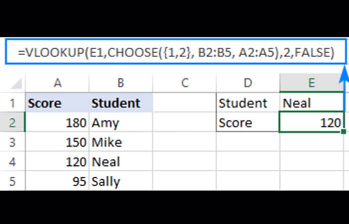
Suppose you have a list of scores in column A, the students' names in column B, and you want to retrieve the score of a particular student. Since the return column is to the left of the lookup column, a normal VLOOKUP formula returns the #N/A error.

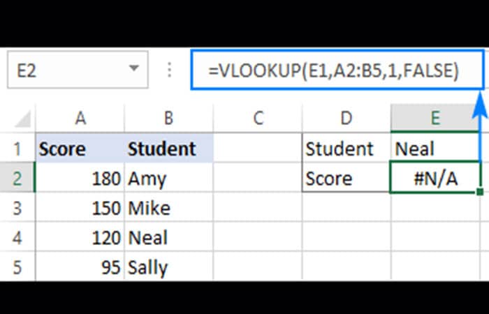
To fix this, use the CHOOSE function to swap the column positions, telling Excel that column 1 is B and column 2 is A:

=CHOOSE({1,2}, B2:B5, A2:A5)

Because we provided an array of {1,2} in the index_num argument , the CHOOSE function accepts ranges in the value arguments (normally, it doesn't). Now, embed the above formula in the table_array argument of VLOOKUP :

=VLOOKUP(E1,CHOOSE({1,2}, B2:B5, A2:A5),2,FALSE)

This will perform a left search without any problems!

The Choose to Return Next Business Day formula

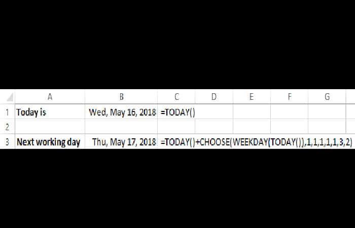
If you're not sure whether you should go to work tomorrow or you can stay home and enjoy your well-deserved weekend, Excel's CHOOSE function can figure out when the next work day is. Assuming your work days are Monday through Friday, the formula is as follows:

=TODAY()+CHOOSE(WEEKDAY(TODAY()),1,1,1,1,1,3,2)

Difficult at first glance, upon closer inspection the logic of the formula is easy to follow:

WEEKDAY(TODAY()) returns a serial number corresponding to today's date, ranging from 1 (Sunday) to 7 (Saturday). This number goes into the Index_num argument of our CHOOSE formula.

Value1 – value7 (1,1,1,1,1,3,2) determines how many days to add to the current date. If today is Sunday – Thursday (index_num 1 – 5), add 1 to return the next day. If today is Friday (index_num 6), add 3 to return the next Monday. If today is Saturday (index_num 7), add 2 to return the next Monday again. Yes, it’s that simple.

Choose formula to return a custom day/month name from date

In situations where you want to get a day name in the standard format, such as the full name (Monday, Tuesday, etc.) or the short name, you can use the TEXT function as explained in this example: Get the day of the week from the date in Excel.

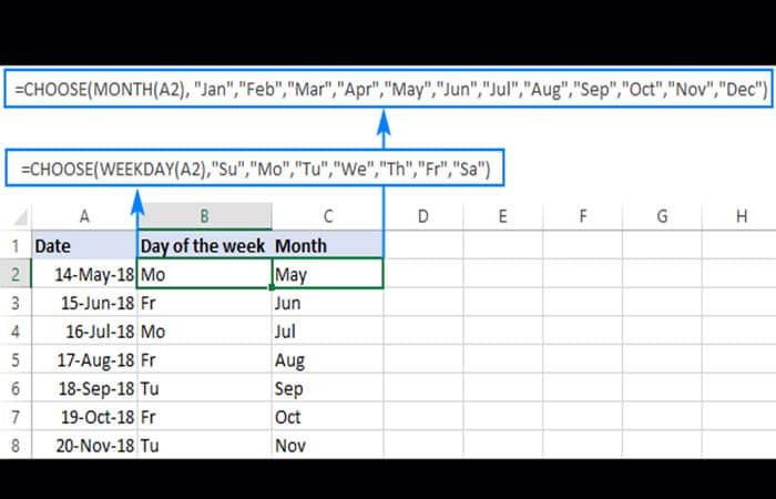
If you want to return the name of a day of the week or a month in a custom format, use Excel's CHOOSE function as follows. To get a day of the week:

=CHOOSE(WEEKDAY(A2),»Su»,»Mo»,»Tu»,»We»,»Th»,»Fr»,»Sa»)

To get a month:

=CHOOSE(MONTH(A2), «Jan»,»Feb»,»Mar»,»Apr»,»May»,»Jun»,»Jul»,»Aug»,»Sep»,»Oct»,»Nov »,»Dec»)

Where A2 is the cell containing the original date.

Check out: Data Bars in Excel. What They Are and How to Add Them

Final thoughts

We hope this tutorial has given you some ideas on how you can use Excel's CHOOSE function to improve your data models. Thanks for reading and we hope to see you back here next week! If you enjoyed the tutorial, please let us know what you think in the comments section. Remember that there are many things you can use this function for, you just need to adapt the data in your formula.