Examples of RANK Functions in Excel, 2021 Guide

Do you want to know how to use the RANK functions in Excel? On this occasion we will give you some examples of this excellent function. You can use the RANK function in Excel to compare numbers with other numbers in the same list. Do you want to know more? We invite you to continue reading.

How to use the RANK function

Now, let's look at how RANK Functions work in Excel. For example, if you give the RANK function a number and a list of numbers, it will tell you the rank of that number in the list, either in ascending or descending order.

Here you can learn about: How to Copy an Excel Sheet to Another Workbook – Tutorial

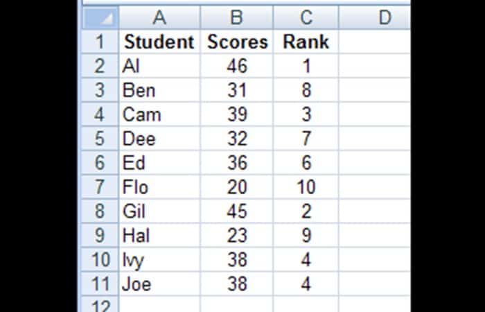
In the screenshot below, there is a list of test scores for 10 students, in the cells B2:B11.

• Step 1:: To find the score range of the first student in cell B2, enter this formula in cell C2:

=RANK(B2,$B$2:$B$11)

• Step 2:: Then copy the formula from cell C2 to cell C11, and the scores will be sorted in descending order.

RANK Function Arguments in Excel

There are 3 arguments for the RANK functions in Excel, which are:

1. Number: In the example above, the number to sort is in cell B2
2. Ref: When you want to compare the number with the list of numbers in the cells $B$2:$B$11. Use an absolute reference ($B$2:$B11), instead of a relative reference (B2:B11) so that the reference range remains the same when you copy the formula to the cells below.
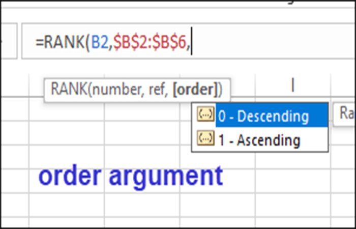
3. order: (optional) This argument tells Excel whether to sort the list in ascending or descending order.
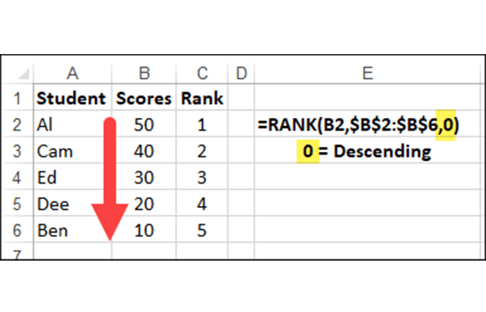
   1. Use zero, or leave this argument empty, to find the range in the list in descending order. In the example above, the order argument was left blank to find the range in descending order. =RANK(B2,$B$2:$B$11)
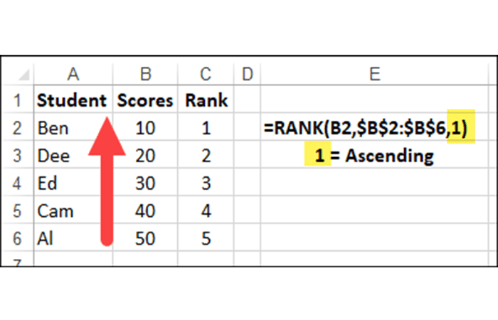
   2. For ascending order, enter a 1 or any other number except zero. If you were comparing golf scores, you might enter a 1 to sort in ascending order. =RANK(B2,$B$2:$B$11)

RANGE Function order

In RANK functions in Excel, the third argument (order) is optional. The order argument tells Excel whether to sort the list in ascending or descending order.

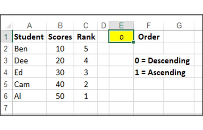
Descending order in RANK functions in Excel

If you use zero as the order setting, or if you do not use the third argument, the range is set to descending order.

• The number bigger gets a rank of 1
• The fifth largest number gets a rank of 5.

Ascending order in RANK functions in Excel

If you use a 1 as the order setting, or if you enter any number except zero As a third argument, the sorting is set in ascending order.

• The number smaller gets a rank of 1
• The fifth smallest number gets a rank of 5.

Flexible formula in RANK functions in Excel

Instead of typing the rank argument number into RANK functions in Excel, use a cell reference to create a flexible formula.

For example: writes a 1 in cell E1 and links cell E1 to the order argument.

NOTE: : you must be sure to use an absolute reference ( $ E $ 1 ), if the formula will be copied to other rows. If you use a relative reference (E1), the reference will change in each row.

=RANK(B2,$B$2:$B$6,$E$1)

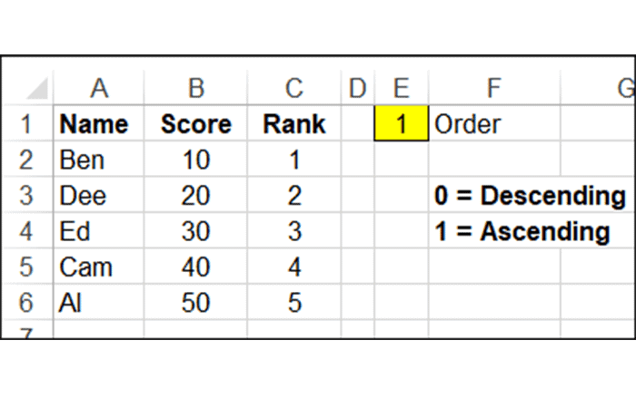
By linking to a cell, you can quickly see different results, without changing the formula. Type a zero in cell E1 or delete the number and the range will change to Descending Order.

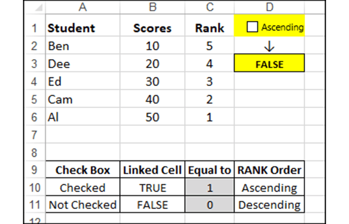
Use a checkbox in RANK functions in Excel

For the sorting option, there are only 2 options: ascending or descending. To make it easier for people to change the order, use a checkbox to enable or disable ascending order.

• If ON, the RANK order will be Ascending.
• If OFF, the RANK order will be Descending.

RANK Function Loops in Excel

What happens to the ranking if some of the scores are tied? Excel will skip subsequent numbers, if necessary, to show the correct range.

• In this example above, the last two scores on the list are the same: 38. The two students, Ivy and Joe, are ranked 4th.
• The next highest score, Ed's score of 36, was ranks sixth, not in the fifth, because there are 5 students ahead of him.

Breaking ties with RANK functions in Excel

In some cases, ties are not allowed, so you must find a way to break the tie.

In this example, you can track the number of minutes each student worked on the test and use that time to break any ties. If scores are tied, the student who takes the least amount of time to complete the test will be ranked ahead of the other student with the same score.

Calculate decimal amount for scores linked with RANK functions in Excel

• Step 1:: Add the test times in column C and a TieBreak formula in column E.
  • =IF(COUNTIF($B$2:$B$11,B2)>1,
    RANK(C2, $C$2: $C$11,1)/100,0)

How the Tiebreaker Formula Works in RANK Functions in Excel

The Tiebreaker formula uses the functions COUNTIF and RANGE, wrapped with a SI function, to see if a decimal tiebreaker amount should be added to the original Range.

• Step 1:: First, the TieBreak formula checks if there is more than one instance of the number in the entire list: IF(COUNTIF($B$2:$B$11,B2) > 1
• Step 2:: If there is more than one instance, sort the times in order upward, because a lower time is better:RANK (C2, $C$2: $C$11, 1)
• Step 3:: Next, divide that amount by 100 to get a decimal amount. Later, you will add this decimal amount to the original range.

Nota: The divisor, 100, could be changed to another number, if you are working with a longer list.   / 100

• Step 4:: Finally, to complete the IF function, if there is only one AA Rank instance, the result of the TieBreak is zero. (0)

Calculate the final ranking with RANK functions in Excel

After calculating the decimal tiebreaker amounts, you can add the results of the RANK function to the TieBreak results to obtain the final standings.

In this example, two students tied for fourth place.

• It took Joe 27 minutes to complete the test and his time ranked fifth.
• It took Ivy 29 minutes to complete the test and her time ranked ninth.

The Tie Break formula adds a decimal of 0.09 to Ivy's score and 0.05 to Joe's score. In the final standings, Joe, with 4.05, ranks above Ivy, with 4.09.

Split earnings for a tied rank

In a tournament, instead of breaking ties, you may want to split the winnings between tied players, if you are awarding a cash or points prize. If 2 or more players have the same rank, they will split the prize amount available for that rank, up to the next occupied rank.

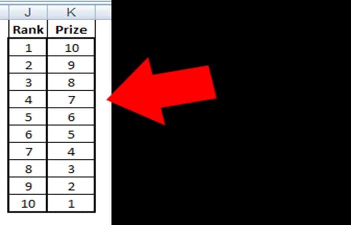
Below is a sample prize table, showing the amount awarded for each rank. In this example, if 3 players are at rank 1, they would split the total amount (10 + 9 + 8 = 27) for ranks 1, 2 and 3.

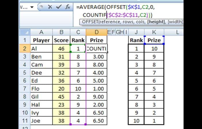
Each of the 3 players in rank 1 wins 9 (27/3 = 9) and the player with the next highest score would be ranked 4th and win 7.

Calculate Divided Amount Using RANK Functions in Excel

To divide the prize amount between tied players, the prize formula uses the AVERAGE function, With the SHIFT function to find the range of cells to average. This formula is entered in cell D2 and copied to cell D11.

=AVERAGE(OFFSET($K$1,C2,0,COUNTIF($C$2:$C$11,C2)))

How the Prize Formula Works with RANK Functions in Excel

The prize formula uses the AVERAGE function, With the SHIFT function to find the range of cells to average.

• Step 1:: The AVERAGE function will calculate the amount for each player, based on a specific range of cells: AVERAGE (
• Step 2: The OFFSET function returns the range with the quantities to use for the average: OFFSET (
• Step 3: In the OFFSET formula, the first argument is the reference cell. In this example, that is cell K1, the Prize Amounts column header.$K$2,
• Step 4: In OFFSET formula, the second argument is the number of rows down from the Reference cell, that the cells to average begin. Ranges are listed in ascending order, so for Range of 1, the cells to average would begin 1 row down from the Reference cell of $K$1. The first player's rank is in cell C2, so refer to that in the formula C2,
• Step 5: In the OFFSET formula, the third argument is the number of columns to the right of the reference cell, which the cells to average begin in. You want to find amounts in the same column, so the number is zero 0,
• Step 6: In the OFFSET formula, the fourth argument is the number of rows to include in the range. This should be the number of players who are tied for that range. The COUNTIF function will count the instances of the range in column C, that are equal to the range in C2 IF ($C$2:$C$11,C2)

RANK Functions in Excel with IF

Instead of using the RANK function to compare a number to an entire list of numbers, you may need to rank a value within a specific subset of numbers.

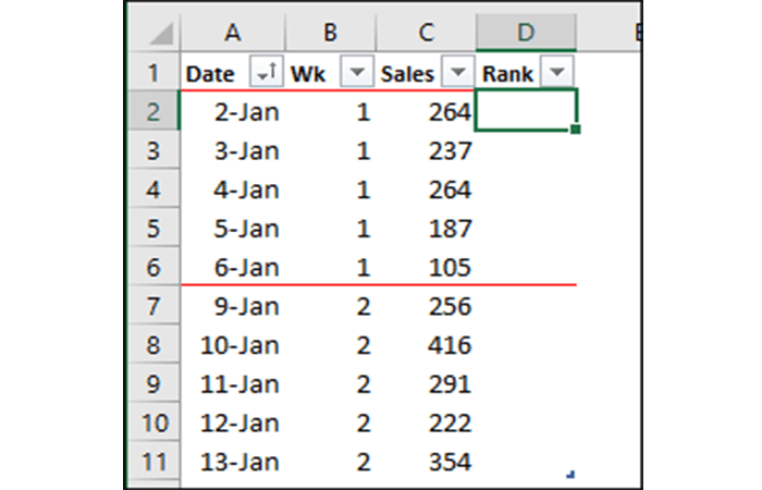
E.g., ranks each day's sales compared to other days in the same week. In the screenshot below, there are sales records for two weeks.

1. January 2nd and 4th have the highest sales in week 1, so they should have a rank of 1.
2. In week 2, January 10th has the highest sales, so it should have a rank of 1 for that week.

Without RANK IF function

There is no RANKIF function, but you can use the COUNTIF function to calculate the rank based on items with the same week number.

Enter this formula in cell D2 and copy it to the last row with data: =COUNTIF([Wk], [@Wk], [Sales], ">" and [@Sales]) + 1

How it works

The first criterion in the formula checks other sales with the same week number:

=COUNT.SE([Wk], [@Wk]

The second criterion looks for items with a higher quantity in the Sales column.

[Sales], «>» and [@ Sales])

Then, 1 is added to that number, to get the ranking.

+1

For example, in week 1, look at sales from January 3 to 237.

• There are 2 dates with higher sales in week 1: January 2 and January 4
• Add 1 to that number, and January 3rd has a range of 3

You may also be interested in reading about: How to Group a Pivot Table by Months in Excel

As you can see, these are examples of the RANK functions in Excel. This is a very effective method if you want to make comparisons quickly. We only recommend that you practice so that it comes naturally to you. We hope we have helped you.